
Baroclinic Rossby waves have long been known to play an important role in the spin-up of the ocean (Anderson and Gill 1975) and so their apparent direct observation through satellite altimetry measurements of global sea surface height (SSH) (Chelton and Schlax 1996) was a well celebrated result. These early observations were shown to differ in their predicted phase speed from linearized quasi-geostrophic theory which motivated numerous attempts to modify the classical theory (e.g., Killworth et al. (1997); Tailleux and McWilliams (2001); Killworth and Blundell (2005)). However, subsequent observations from higher resolution SSH fields constructed from multiple satellite altimeters have cast doubt on the original interpretation of the observations as linear waves (Chelton et al. 2007, 2010). The enhanced observations now show more eddy-like characteristics that remain coherent structures for long durations with opposing meridional deflections of cyclones and anticyclones, and suggest a significant degree of nonlinearity through several non-dimensional parameters. Motivated by these observations, we examine the basic characteristics of Rossby waves and eddies in a standard quasi-geostrophic setting.
Satellite Observations
The following is an animation of sea surface height from satellite altimetry measurements that has been filtered to isolate the westward propagating features that are clearly visible in much of the ocean (Chelton et al. 2007, 2010).
The figure below shows the zonal frequency-wavenumber spectra for sea surface height from the satellite altimetry data along 24 N in the western subtropical Pacific Ocean.
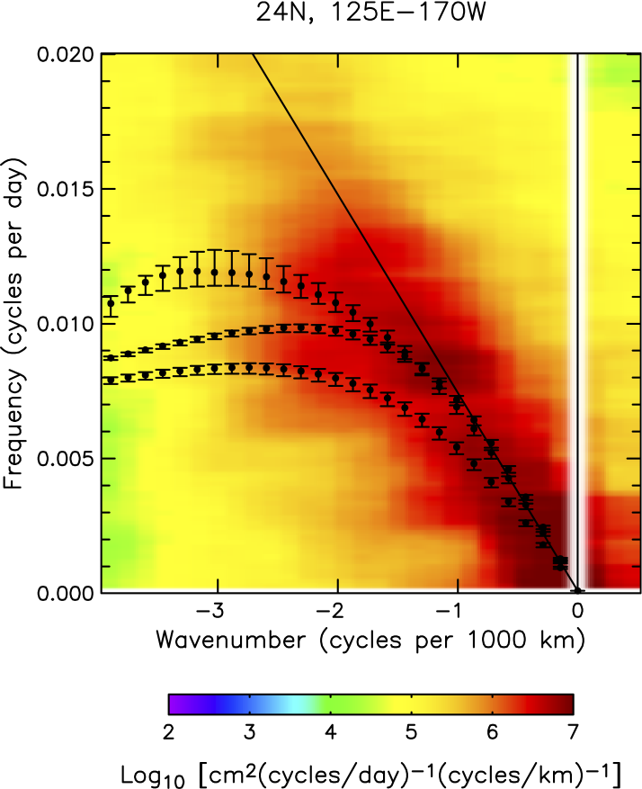
The three dispersion relations shown are from standard Rossby wave theory, the rough bottom topography theory of Tailleux and McWilliams (2001) and the vertical shear-modified theory of Killworth et al. (1997) extended to the case of nonzero zonal wavenumber (Fu and Chelton 2001), in order of increasing frequency.
Numerical Model
We consider both linear ( \(\beta^{-1}=0\) ) and nonlinear ( \(\beta^{-1} \neq 0\) ) quasi-geostrophic theory in a reduced-gravity shallow-water model,
\begin{equation}
\label{eqn:QGChap2}
\frac{\partial}{\partial t} \left( \nabla^2 \eta – \eta \right) + \frac{\partial \eta }{\partial x} + \beta^{-1} \cdot J \left( \eta, \nabla^2 \eta \right) = 0
\end{equation}
where the dimensionless variable \(\eta(x,y,t)\) is a sea-level height perturbation scaled by a representative value \(\eta_0\), and the Jacobian is defined as \(J(a,b) = a_x b_y – a_y b_x\). The nondimensional coefficient \(\beta^{-1} = \frac{U}{\beta_0 L_R^2}\) where \(U = g \eta_0/(f_0 L_R)\) is the geostrophic velocity scale associated with \(\eta_0\), \(g\) is the acceleration of gravity, \(\beta_0\) is the variation of the Coriolis parameter and \(L_R\) is the Rossby radius of deformation.
Eddy Seeding Experiment
To compare the wavenumber-frequency spectra of observations with those of the linear and nonlinear models, a basin 8300 km by 3850 km with periodic boundary conditions was seeded with Gaussian eddies. The eddy seeds were of varying amplitude (both positive and negative), horizontal length scales and with a frequency of occurrence matching the statistics of the observed eddies in a region of the subtropical North Pacific (Chelton et al. 2010). The simulation was run and continuously seeded with these eddies throughout the domain for 150 years. To prevent signals from crossing the boundaries, a 400 km thick sponge layer was added to all four sides of the basin.
The following two animations show eleven years of the eddy seeding experiments, starting at day 1475.
The linear animation shows an evolving interference pattern created by the dispersion of the Gaussian seeds.
The same eddy seeds evolved with nonlinear dynamics are qualitatively very different. Individual eddies remain coherent for long durations and there’s a clear tendency towards longer wavelengths.
The zonal frequency-wavenumber spectra in the figure below show very different behaviors between the two models.
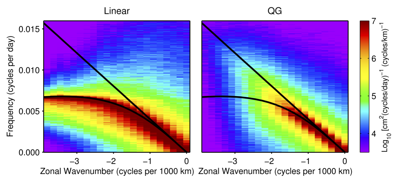
For the linear model, the variance is restricted to frequencies below the meridional wavenumber \(l=0\) of the zonal Rossby wave dispersion relation. This is consistent with theory, as waves with given zonal (\(k\)) and non-zero meridional wavenumbers (\(l\neq0\)) have frequencies that remain below the frequency for \(l=0\). The power distributions for the nonlinear model are substantially different than the linear model. The signals are essentially non-dispersive for lower wavenumbers for both models, while the energy at higher wavenumbers remains centered along the same non-dispersive slope for the nonlinear model but not the linear model.
The zonal frequency-wavenumber spectrum of the nonlinear model is very similar to that of the observations, while the linear model fails to explain the non-dispersive structure observed. As such, linearized quasi-geostrophic theory is not a viable theory to explain the observed westward propagating features.
Waves versus Eddies
The following two animations show the evolution of an initially Gaussian sea surface height of amplitude 15 cm and length scale 80 cm. The first animation uses the linear form of the equation with \( \beta^{-1}=0 \), while the second animation uses the value appropriate for the first baroclinic mode at latitude 24, \( \beta^{-1} =7.5\). Black contours are drawn at sea-level to emphasize the peaks and troughs of the resulting interference pattern.
The eddy evolved under linear dynamics is dominated by Rossby wave interference patterns, although the sea surface maximum can still be observed to propagate westward. After 365 days the amplitude of the eddy is only 3 cm.
The Gaussian modeled with the nonlinear equation also shows Rossby wave interference patterns, but is dominated by the coherent westward propagating sea surface maximum. The nonlinear anticyclonic eddy also shows a much slower amplitude decay rate (its amplitude is still 11 cm after 365 days) and an equatorward deflection (McWilliams and Flierl 1979), both qualitatively consistent with the observations reported by Morrow et al. (2004) and Chelton et al. (2007, 2010).
Fluid Transport
In order to investigate the advective properties of the eddies, both a passive tracer and floats were added to the model. The passive tracer, \( W(x,y,t) \), is a scalar field with no sources or sinks initialized with the value of its initial \( x \) position and then allowed to evolve with the equation,
\[
\frac{\partial W}{\partial t} + u \frac{\partial W}{\partial x} + v \frac{\partial W}{\partial y} = 0.
\]
These animations show a tracer field initially varied in the zonal, \( x \), direction which is then advected by the the linear and nonlinear eddies. The same black contours of sea-level are drawn over the tracer field as was done with the the sea surface height animations above.
The eddy evolved under linear dynamics transports some fluid more than 1000 km from its origin.
Now compare this to the eddy evolved with nonlinear dynamics below. In this case the contour of zero relative vorticity is drawn in black and defines the boundary of what is called the eddy core. The instantaneous trapped fluid contour is drawn in gray and is determined by transforming into coordinates co-moving with the eddy and finding the largest closed contour of height or pressure. The region between the contour of zero relative vorticity and the trapped fluid contour is defined as the eddy ring.
The nonlinear eddy transports fluid very differently than the linear eddy. At any point during the eddy’s lifetime, 100% of the fluid in the core is from the initialization location. This is in contrast to the ring, which does not well describe the boundary retaining fluid. The ring entrains and sheds fluid throughout its lifetime, moving some parcels of fluid hundreds of kilometers and others thousands of kilometers.
Potential Vorticity
The quasigeostrophic potential vorticity equation is a conservation equation. Conservation of potential vorticity for a fluid parcel has contributions from three terms: planetary vorticity, relative vorticity and vortex stretching.
\begin{equation}
\label{pv_conservation}
\frac{d}{dt} \left[ \underbrace{\beta_0 y}_{\textrm{planetary vorticity}} + \underbrace{\frac{g}{f_0}\nabla^2 \eta}_{\textrm{relative vorticity}} – \underbrace{\frac{f_0}{D} \eta}_{\textrm{vortex stretching}} \right] = 0
\end{equation}
The animation below shows the total potential vorticity of the nonlinear monopole. The units of vorticity are normalized by \(\beta*1000\) essentially indicating where a fluid particle would come to rest if its sea-surface height and relative vorticity were zero. Note that the frame is moving.
The next animation shows the same isolines of potential vorticity, but this time they are drawn on top of the passive zonal tracer.