
This is a summary of the paper published in the Journal of Atmospheric and Oceanic Technology in March 2020. All of the associated code and documentation is publicly available.
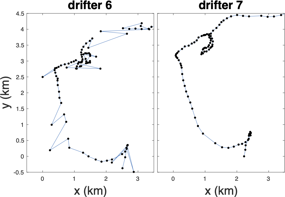
In the summer of 2011 an array of drifters were deployed in the Sargasso Sea as part of an ONR funded project to study submesoscale motions. Submesoscale motions are defined to occur at spatial scales of around 1-10 km and time scales of hours to days; however, although GPS receivers can record to accuracies of a few meters, the drifters deployed showed numerous outliers as can be seen below.
With the ultimate goal to use the drifters to understand submesoscale flow, there are a few issues that we need to deal with first.
- How to we identify and handle outliers?
- How do we smooth and interpolate the GPS data to get the best possible fit?
- How does the process of interpolation affect the signal?
This last question is really important—because our interest is in the short time/high frequency part of the signal, we need to be very careful that interpolation and smoothing isn’t directly affect the part of the signal that we are analyzing.
Smoothing splines
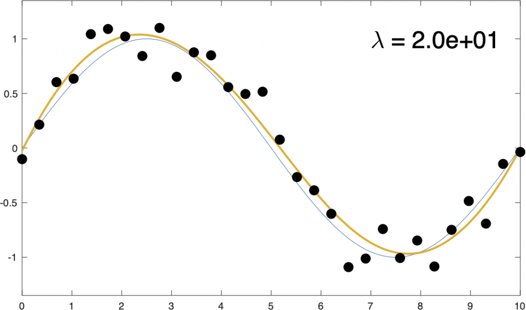
The approach taken here is to use a collection of b-splines, essentially one for each data point, and then apply a smoothing penalty function. Check out the documentation for quick practical overview of b-splines. Conceptually, we are creating a linear mapping from our observations, \( \mathbf{x} \), to new smoothed points, \( \hat{x} \), with smoothing matrix, \( \mathbf{S}_\lambda \) for some parameter \( \lambda \). That is, \( \hat{x}=\mathbf{S}_\lambda \mathbf{x} \). Changing the value of \( \lambda \) changes how smooth the resulting fit is,
How do we set the smoothing parameter \(\lambda\)? Easy! Craven and Wahba 1978 showed that you can simply minimize the expected mean-square error.
\[ \textrm{MSE}(\lambda) = \frac{1}{N} || \left( \mathbf{S_\lambda} – I \right) \mathbf{x} ||^2 + \frac{2 \sigma^2}{N} \textrm{Tr}\, \mathbf{S_\lambda} – \sigma^2 \]This works remarkably well as can be seen in the figure below,
This methodology can be implemented in just a few lines using code, e.g.,
spline = SmoothingSpline(x,y,NormalDistribution(sigma));So why can’t we just use the methodology as is for the GPS drifters?
GPS error distribution
In the previous example we assumed that the errors had a Gaussian distribution, but GPS errors follow a t-distribution. Finding the error distribution is as simple as turning on your GPS and leaving it in the same spot for a few days. Because the errors are (eventually) relatively uncorrelated, by the central limit theorem, the mean position is pretty close to your true position.
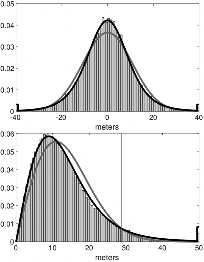
(top) The position error distribution of the motionless GPS. The gray or black curves are the best-fit Gaussian or t distribution, respectively. (bottom) The distance error distribution with the corresponding expected distributions from the Gaussian and t distributions. The vertical line in the bottom panel shows the 95% error of the t distribution
So now, we simply need to adjust the spline fitting process to use a t-distribution instead of a normal distribution. In code, this is just,
spline = SmoothingSpline(x,y,StudentTDistribution(sigma,nu));which can immediately be done independently for the x and y direction of drifter 7, which doesn’t show any outliers.
Outliers
The key to handling outliers to recognize that their errors follow a different distribution than the expected GPS distribution. This idea is then there are two relevant distributions, the GPS distribution and an outlier distribution, as shown in the figure below,
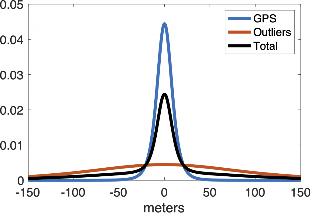
The observed distribution of errors (black) is actually a weighted sum of the expected GPS error distribution (blue) and some unknown outlier distribution (red) with significantly larger variance.
There are a number of possible approaches that use this basic model to improve the fit, including trying to directly model the outlier distribution. However, with some experimentation, we found that the most robust thing to do is arguably the simplest thing: simply exclude outliers from the expected mean square error calculation, where an outlier is defined as a point with less than 1% odds of occurring.
So, rather than using the total expected variance \( \sigma^2 \) in the equation for \( \textrm{MSE} \) as above, instead use variance over some expected range,
\[ \sigma_\beta^2 = \int_{\textrm{cdf}^{-1}(\beta/2)}^{\textrm{cdf}^{-1}(1-\beta/2)} z^2 p_{\textrm{noise}}(z) \, dz \]where \( \beta \) is a value of about 1/100. This also means you need to discard all rows (and columns) of \( \mathbf{S}_\lambda \) where \( \left( \mathbf{S}_\lambda – I\right)\mathbf{x} < \textrm{cdf}^{-1}(\beta/2) \) or \( \left(\mathbf{S}_\lambda - I\right)\mathbf{x} > \textrm{cdf}^{-1}(1-\beta/2) \) when actually minimizing for the expected mean-square error.
So how does this work in practice? In the left panel of the movie below we show the effect of varying the smoothing parameter \(\lambda\) where the t-distribution is assumed for the errors. In the right panel we show the value of the expected mean-square error for cross-validation (“CV MSE”, blue) and the ranged expected mean-square error (“Ranged MSE”, red). As the smoothing parameter \(\lambda\) increases you can see the spline fit pull away from some obvious outlier points.
The minimum of the ranged MSE is at a higher value of \(\lambda\) than the CV MSE and our test suggest that the ranged MSE is the better estimator. Note that as \(\lambda\) continues to increase to values above the ranged MSE minimum, the spline starts to become over-tensioned. You can see this visually as the spline systematically pulls to one side of consecutive points—this is not realistic because the errors are not correlated at this time.
The code for this is also very simple,
spline = GPSSmoothingSpline(t,lat,lon);and essentially just projects the latitude and longitude onto transverse Mercator coordinates, before applying the methodology described above.
How does interpolation and smoothing affect the signal?
One of the most important results from this study is quantifying how many degrees of freedom are lost to smoothing and interpolating. If your sampling time between observation is \( \Delta t \) then your Nyquist frequency is given as,
\[ f \equiv \frac{1}{2 \Delta t} \]which sets the highest resolvable frequency. However, the process of smoothing causes you to lose some degrees of freedom. We show in the manuscript that your effective Nyquest frequency is given by
\[ f^\textrm{eff} \equiv \frac{1}{2 n_\textrm{eff} \Delta t} \]where \( n_\textrm{eff} \) is the effective sample size of the variance of the mean defined by
\[ \frac{\sigma^2}{n_\textrm{eff}} = \frac{1}{N} \textrm{Tr} \, \left( \mathbf{S}_\lambda \mathbf{\Sigma} \right). \]To show how this works, we generate a signal (black) and then contaminate it with noise (red). We then do a spline fit to three different subsampled the signal where we include all points (blue), every 10 points (red) and every 100 points (blue). The top panel of the figure below shows the resulting frequency spectrum. In the bottom panel we then compute the coherence of the interpolated signal and the true uncontaminated signal.
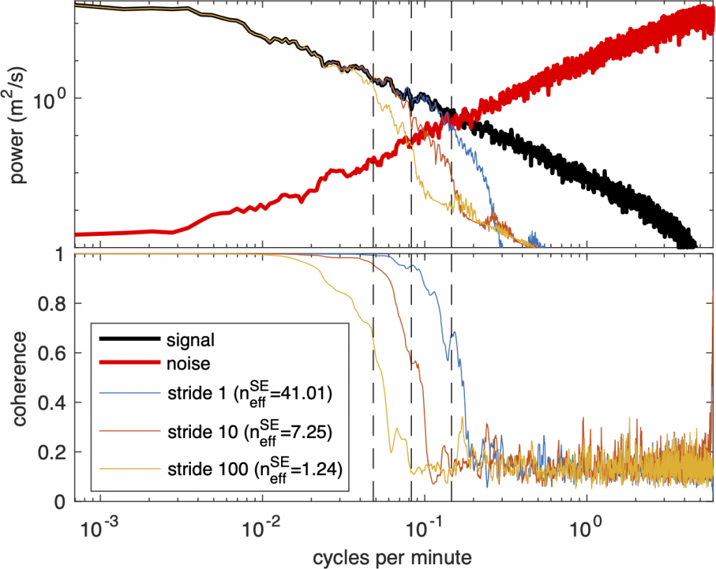
The key takeaway from this figure is that they coherence goes to zero for frequencies above the effective Nyquist. This means that any `signal’ at higher frequencies is actually just noise. Thus, any analysis should be limited to frequencies below the effective Nyquist.
A related issue is the the degree (or order) of b-spline that should be used. The degree (S) of a spline sets the number of non-zero derivatives, e.g., the usual cubic spline has three non-zero derivatives. To test the effect of change S, we use splines of different degree to fit to the same data, the resulting spectra are plotted below.
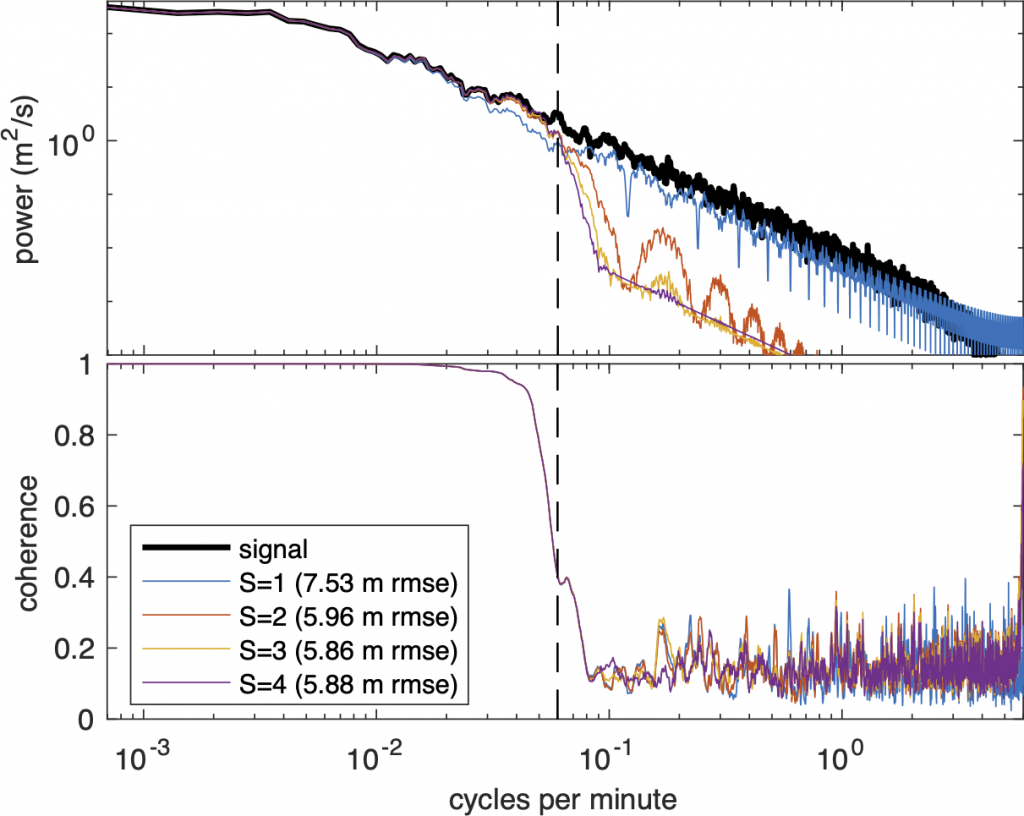
At first glance it would appear that the S=1 spline fit is best—after all, its high frequency slope matches that of the real data (black). However, note that its coherence drops to zero at the same frequency as the other spline degrees and that it has a higher root mean-square error (rmse). What’s happening is that S=1 spline is essentially generating random noise at higher frequencies, creating the illusion of a better fit, while in practice actually increasing error. In conclusion, you should use a relatively high degree b-splines for your fit, while limiting your analysis to frequencies below the effective Nyquist, as mentioned above.
Other notes
The manuscript includes many other results and the code is fairly robust. A few other highlights include,
- an introduction to b-splines and interpolating splines,
- a physical interpretation of what the smoothing spline is doing,
- a method for directly relating \( \lambda \) to the rms velocity of the signal,
- an approach to handling bivariate data (such as the drifter data),
- numerical methods for evaluating to non-Gaussian pdfs.